Bivariate Palettes
Christopher Prener, Ph.D. and Branson Fox
2025-09-01
Source:vignettes/bivariate_palettes.Rmd
bivariate_palettes.RmdOne of the important aspects of cartography and data visualization is
color choice. This vignette illustrates the palettes included with
biscale, provides an overview of palette manipulation
tools, and describes the revised approach to utilizing custom
palettes.
Included Palettes
As of v1.0.0, biscale supports a dozen built-in
palettes and expanded ability to utilize custom palettes. For five of
these palettes, there are both “primary” versions and “legacy
versions.”
Primary Palettes
All of the primary palettes listed here can be used with two-by-two
(dim = 2), three-by-three (dim = 3), and
four-by-four (dim = 4) maps. The palettes that contain a
2 at the end of their name are visually similar to the
original, “legacy” palettes (see below) but utilize slightly different
hex values for colors.
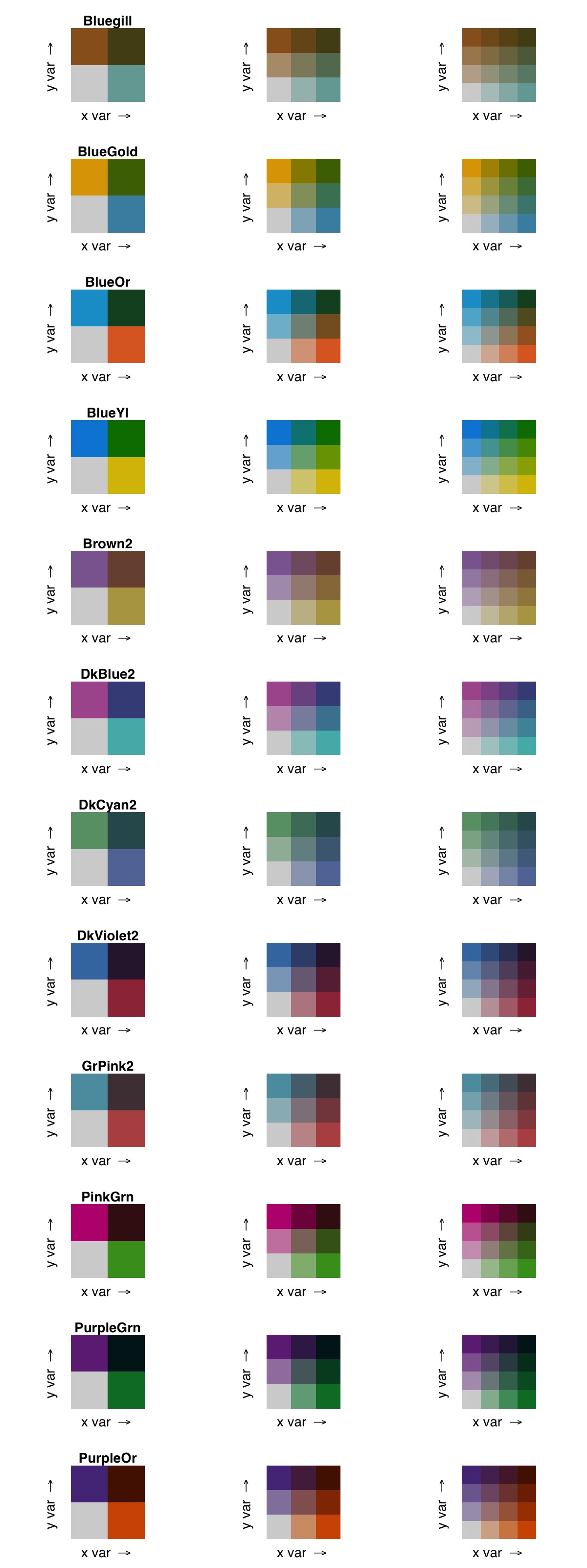
Most of the newly added palettes not based on legacy designs were adapted from earlier work by Branson Fox.
Legacy Palettes
To ensure compatibility with scripts written with older versions of
biscale, the original five palettes included in the package
are still available. They can be used only for two-by-two
(dim = 2) and three-by-three (dim = 3)
maps.
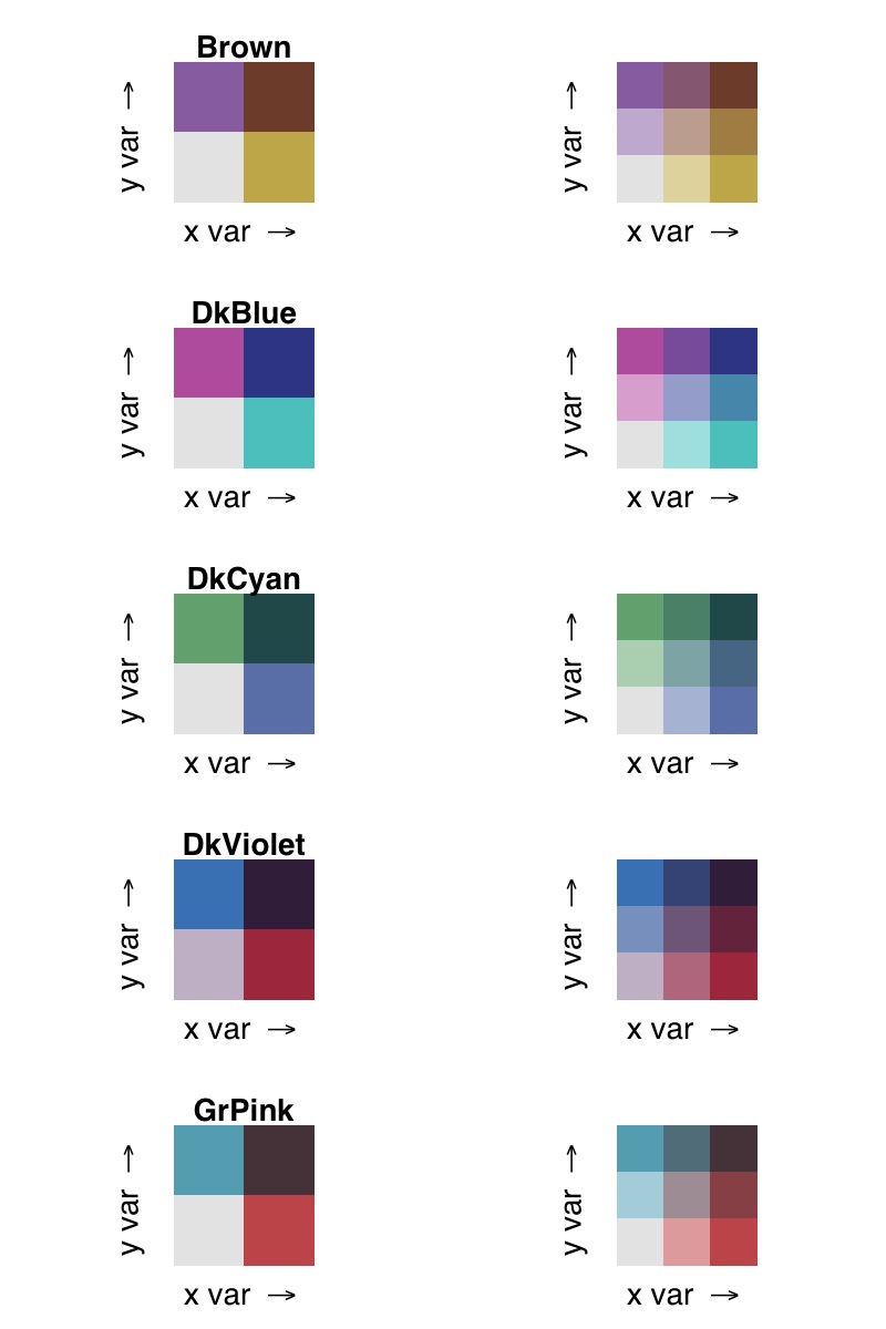
The "DkViolet" palette was created by Timo
Grossenbacher and Angelo Zehr, and the other four palettes were
created by Joshua
Stevens.
Palette Manipulations
In order to facilitate even greater flexibility with palettes,
biscale functions include two additional arguments to
manipulate their arrangement.
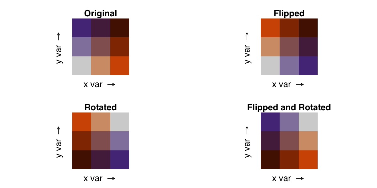
“Flipping axes” will invert the colors assigned to the x and y axes.
Flipping axes is accomplished with the flip_axes
argument:
bi_pal(pal = "PurpleOr", dim = 3, flip_axes = TRUE)“Rotating” the palette (with the rotate_pal argument)
will rotate the colors 180 degrees, resulting in a palette that
highlights low values as opposed to high values. Rotating the palette
rotates the entire color scale 180 degrees. For example:
bi_pal(pal = "PurpleOr", dim = 3, rotate_pal = TRUE)These manipulations can be combined as well, producing a palette that has been both flipped and rotated:
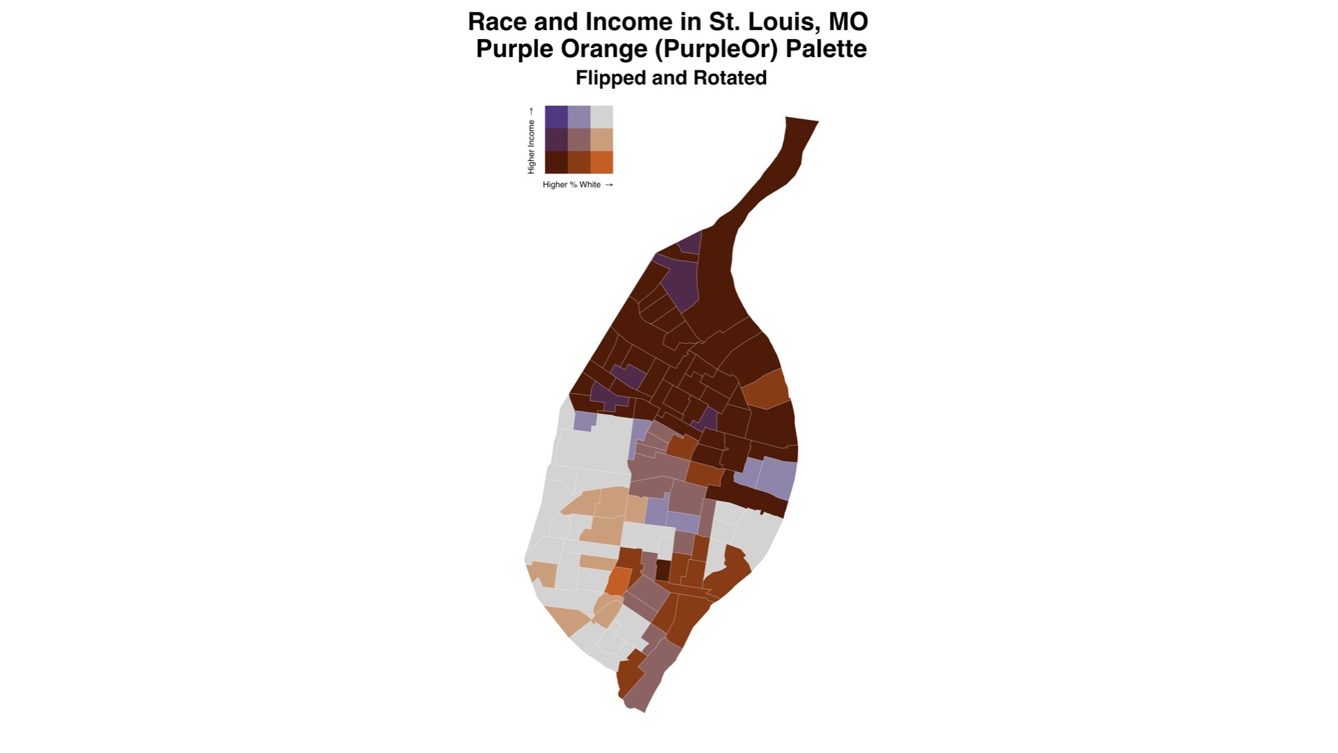
bi_pal(pal = "PurpleOr", dim = 3, flip_axes = TRUE, rotate_pal = TRUE)Together, these changes to bi_pal() result in the
following shifts to the "PurpleOr" palette:
When applied to real world data, these transformations result in subtle (in the case of flipping) or more dramatic (in the case of rotating) differences in maps:
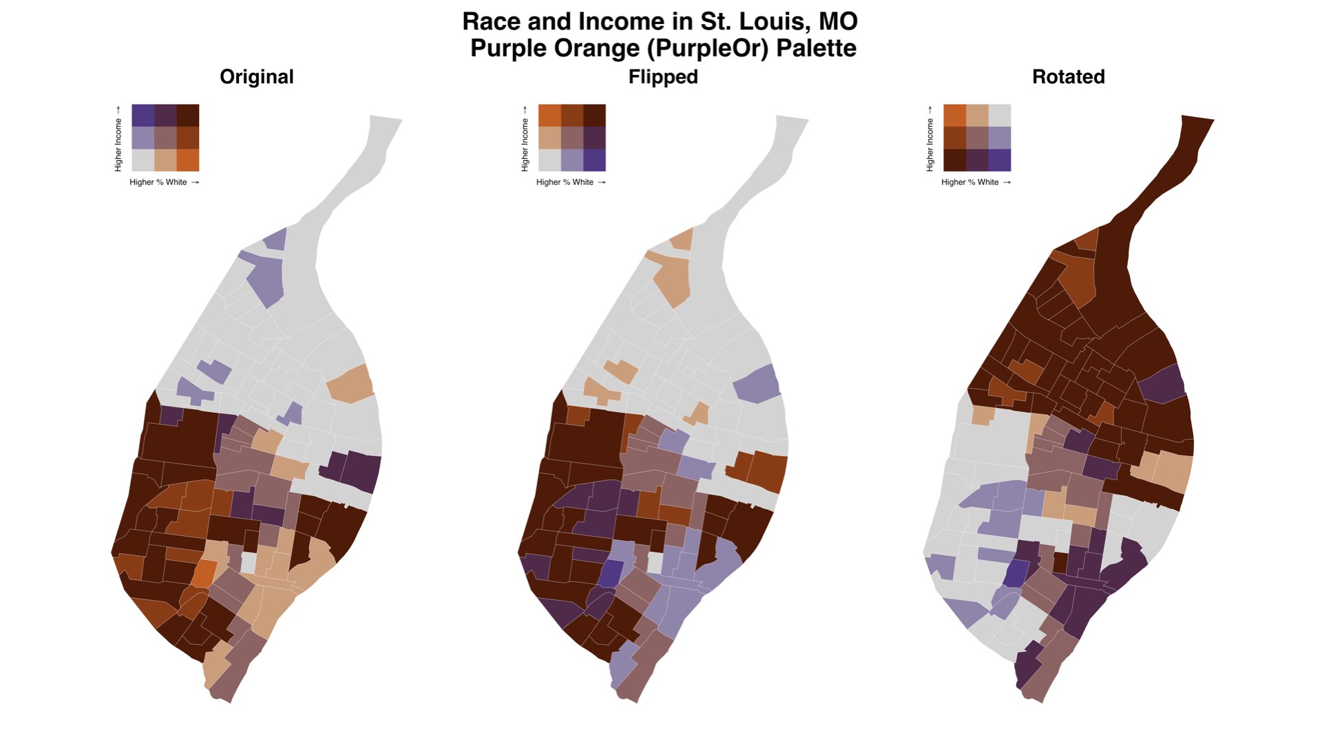
Utilizing both flipping axes and palette rotations also yields a considerable change from the original:
Be careful to ensure that your use of flip_axes and/or
rotate_pal is consistent across
bi_scale_fill()/bi_scale_color() as well as
bi_legend().
Custom Palettes
In addition the built-in palettes described above,
biscale supports custom palettes. As of v1.0.0, the
workflow for using custom palettes is different than prior releases and
the old approach, using bi_pal_manual(), has been
deprecated. We plan to remove bi_pal_manual() in late 2022.
Please update your workflows accordingly.
To create a custom palette, users must create a named vector and supply associated hex values. We recommend checking out Benjamin Brooke’s Bivariate Choropleth Color Generator if you want to experiment with creating your own palettes. Joshua Steves’ blogpost from 2015 also contains tips for creating palettes.
The first example below is a named vector for a two-by-two
(dim = 2) map. The pairs correspond to x,y
coordinates on the legend where the first value is the x
value and the second is the y value. The 1-1
pair is therefore the lower left corner of the legend and, in the
example, the 2-2 pair is the upper right corner. The named
vector should have 4 values in total.
custom_pal2 <- c(
  "1-1" = "#d3d3d3", # low x, low y
  "2-1" = "#9e3547", # high x, low y
  "1-2" = "#4279b0", # low x, high y
  "2-2" = "#311e3b" # high x, high y
)
If you are creating a custom palette for a three-by-three
(dim = 3) map, you need to extend each row and column by 1
so that 3-1 and 3-2 are included in the vector
along with 1-3, 2-3, and 3-3. The
named vector should have 9 values in total.
custom_pal3 <- c(
  "1-1" = "#d3d3d3", # low x, low y
  "2-1" = "#ba8890",
  "3-1" = "#9e3547", # high x, low y
  "1-2" = "#8aa6c2",
  "2-2" = "#7a6b84", # medium x, medium y
  "3-2" = "#682a41",
  "1-3" = "#4279b0", # low x, high y
  "2-3" = "#3a4e78",
  "3-3" = "#311e3b" # high x, high y
)
Finally, for a four-by-four (dim = 4), should be further
extended by 1 so that 4-1, 4-2, and
4-3 are included in the vector along with 1-4,
2-4, 3-4, and 4-4. The named
vector should have 16 values in total.
custom_pal4 <- c(
  "1-1" = "#d3d3d3", # low x, low y
  "2-1" = "#c2a0a6",
  "3-1" = "#b16d79",
  "4-1" = "#9e3547", # high x, low y
  "1-2" = "#a3b5c7",
  "2-2" = "#96899d",
  "3-2" = "#895e72",
  "4-2" = "#7a2d43",
  "1-3" = "#7397bb",
  "2-3" = "#697394",
  "3-3" = "#604e6b",
  "4-3" = "#56263f",
  "1-4" = "#4279b0", # low x, high y
  "2-4" = "#3c5c8b",
  "3-4" = "#373f65",
  "4-4" = "#311e3b" # high x, high y
)
You can preview and validate your named vector using
bi_pal(). For example, we can preview the
custom_pal3 vector created above:
Once you have created your named vector, you can use it any place
where you would ordinarily provide a quoted palette name in
biscale functions. In this example, the
custom_pal3 vector created above is passed to
bi_scale_fill() and bi_legend():
# prep data
data <- stl_race_income
data <- bi_class(data, x = pctWhite, y = medInc, dim = 3, style = "quantile", keep_factors = TRUE)

# draw map
map <- ggplot() +
  geom_sf(data = data, aes(fill = bi_class), color = "white", size = 0.1, show.legend = FALSE) +
  bi_scale_fill(pal = custom_pal3, dim = 3) +
  labs(
    title = "Race and Income in St. Louis, MO",
    subtitle = "Custom Palette"
  ) +
  bi_theme()

# draw legend
legend <- bi_legend(pal = custom_pal3,
                  xlab = "Higher % White ",
                  ylab = "Higher Income ",
                  size = 12)
When custom palettes are passed to biscale functions,
they will be validated to ensure they have the correct number of
entries, have the correct names, and have properly formatted hex
values.
For custom palettes that are two-by-two (dim = 2),
three-by-three (dim = 3), or four-by-four
(dim = 4), the palette manipulations described above can
also be applied:
bi_pal(pal = custom_pal3, dim = 3, flip_axes = TRUE, rotate_pal = TRUE)High Dimensional Palettes
The custom palette workflow not only enables users to bring whatever
color scheme they wish to biscale, but it provides support
for higher dimensional maps (dim = 5 and beyond). Users
should carefully consider the readability of these maps, however, and a
warning to this effect will be generated when using
bi_class(). Users creating high dimensional maps should
also note that flipping and rotating palettes is not supported beyond
dim = 5, and any modifications to the palette must be made
manually.
To create a named vector for a five-by-five (dim = 5)
map, for example, the following named vector could be used:
custom_pal <- c(
  "1-1" = "#d3d3d3", # low x, low y
  "2-1" = "#b6cdcd",
  "3-1" = "#97c5c5",
  "4-1" = "#75bebe",
  "5-1" = "#52b6b6", # high x, low y
  "1-2" = "#cab6c5",
  "2-2" = "#aeb0bf",
  "3-2" = "#91aab9",
  "4-2" = "#70a4b2",
  "5-2" = "#4e9daa",
  "1-3" = "#c098b9",
  "2-3" = "#a593b3",
  "3-3" = "#898ead",
  "4-3" = "#6b89a6",
  "5-3" = "#4a839f",
  "1-4" = "#b77aab",
  "2-4" = "#9e76a6",
  "3-4" = "#8372a0",
  "4-4" = "#666e9a",
  "5-4" = "#476993",
  "1-5" = "#ad5b9c", # low x, high y
  "2-5" = "#955898",
  "3-5" = "#7c5592",
  "4-5" = "#60528d",
  "5-5" = "#434e87" # high x, high y
)