Digitizing Qualitative GIS Data with qualmap

Overview

This package implements a process for converting qualitative GIS data from an exercise where respondents are asked to identify salient locations on a map. This article focuses primarily on the use of the software to digitize these data.

Motivation and Approach

Qualitative GIS outputs are notoriously difficult to work with because individuals’ conceptions of space can vary greatly from each other and from the realities of physical geography themselves. qualmap builds on a semi-structured approach to qualitative GIS data collection. Respondents use a specially designed basemap that allows them free reign to identify geographic features of interest and makes it easy to convert their annotations into digital map features. This is facilitated by including on the basemap a series of polygons, such as neighborhood boundaries or census geography, along with an identification number that can be used by qualmap. A circle drawn on the map can therefore be easily associated with the features that it touches or contains.

qualmap provides a suite of functions for entering, validating, and creating sf objects based on these hand drawn clusters and their associated identification numbers. Once the clusters have been created, they can be summarized and analyzed either within R or using another tool.

This approach provides an alternative to either unstructured qualitative GIS data, which are difficult to work with empirically, and to digitizing respondents’ annotations as rasters, which require a sophisticated workflow. This semi-structured approach makes integrating qualitative GIS with existing census and administrative data simple and straightforward, which in turn allows these data to be used as measures in spatial statistical models.

Cartographica Article

An article describing qualmap’s approach to qualitative GIS has been published in Cartographica. All data associated with the article are also available on Open Science Framework, and the code are available via Open Science Framework and GitHub. Please cite the paper if you use qualmap in your work!

Installation

The easiest way to get qualmap is to install it from CRAN:

install.packages("qualmap")

You can install the development version of qualmap from Github with the remotes package:

# install.packages("remotes")
remotes::install_github("chris-prener/qualmap")

Note that installations that require sf to be built from source will require additional software regardless of operating system. You should check the sf package website for the latest details on installing dependencies for that package. Instructions vary significantly by operating system.

Basics

qualmap is built around a number of fundamental principles. The primary data objects created by qm_combine() are long data rather than wide. This is done to facilitate easy, consistent data management. The package also implements simple features objects using the sf package. This provides a modern interface for working with spatial data in R.

Core Verbs

qualmap implements six core verbs for working with mental map data:

qm_define() - create a vector of feature id numbers that constitute a single “cluster”
qm_validate() - check feature id numbers against a reference data set to ensure that the values are valid
qm_preview() - plot cluster on an interactive map to ensure the feature ids have been entered correctly (the preview should match the map used as a data collection instrument)
qm_create() - create a single cluster object once the data have been validated and visually inspected
qm_combine() - combine multiple cluster objects together into a single tibble data object
qm_summarize() - summarize the combined data object based on a single qualitative construct to prepare for mapping

The order that these functions are listed here is the approximate order in which they should be utilized. Data should be defined, validated and previewed, and then cluster objects should be created, combined, and summarized.

Main Arguments

All of the main functions except qm_define() and qm_combine() rely on two key arguments:

ref - a reference object. This should be an sf object that contains a master list of features that appear in your study. This could a sf object representing all census tracts in a city or county, for example, or a tessellated grid covering the extent of a city.
key - the name of geographic id variable in the ref object to match input values to. This could be a FIPS code, the GEOID variable in most census data, or the OBJECTID of a tessellated grid. Values entered into qm_define() should key values.

Additionally, a number of the initial functions have a third essential argument:

value - the name of the cluster created using qm_define()

Data Preparation

To begin, you will need a simple features object containing the polygons you will be matching respondents’ data to. Census geography polygons can be downloaded via tigris, and other polygon shapefiles can be read into R using the sf package.

Here is an example of preparing data downloaded via tigris:

library(dplyr)   # data wrangling
library(sf)      # simple features objects
library(tigris)  # access census tiger/line data

stLouis <- tracts(state = "MO", county = 510)
stLouis <- mutate(stLouis, TRACTCE = as.numeric(TRACTCE))

We download the census tract data for St. Louis and convert the TRACTCE variable to numeric format.

If you want to use your own base data instead, you can use the st_read() function from sf to bring them into R.

Data Entry

Once we have a reference data set constructed, we can begin entering the tract numbers that constitute a single circle on the map or “cluster”. We use the qm_define() function to input these id numbers into a vector:

cluster1 <- qm_define(118600, 119101, 119300)

We can then use the qm_validate() function to check each value in the vector and ensure that these values all match the key variable in the reference data:

> qm_validate(ref = stLouis, key = TRACTCE, value = cluster1)
[1] TRUE

If qm_validate() returns a TRUE value, all data are matches. If it returns FALSE, at least one of the input values does not match any of the key variable values. In this case, our key is the TRACTCE variable in the sf object we created earlier.

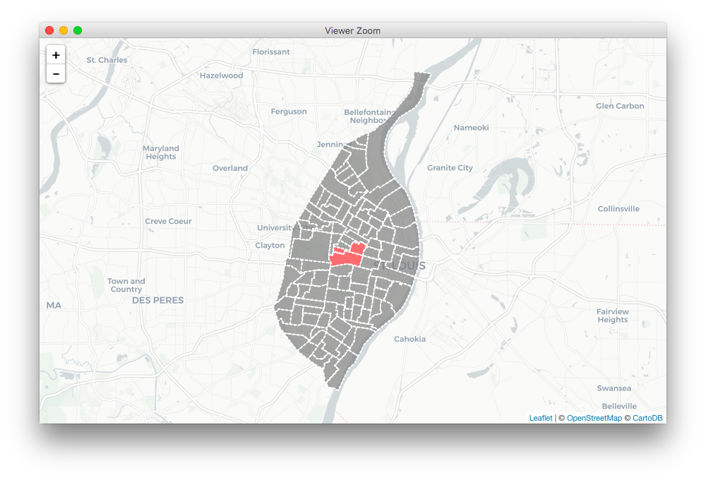
Once the data are validated, we can preview them interactively using qm_preview(), which will show the features identified in the given vector in red on the map:

qm_preview(ref = stLouis, key = TRACTCE, value = cluster1)

Create Cluster Object

A cluster object is tibble data frame that is “tidy” - each feature in the reference data is a row. Cluster objects also contain metadata about the cluster itself: the respondent’s identification number from the study, a cluster identification number, and a category that describes what the cluster represents. Clusters are created using qm_create():

> cluster1_obj <- qm_create(ref = stLouis, key = TRACTCE, value = cluster1, rid = 1, cid = 1, category = "positive")
> cluster1_obj
# A tibble: 3 x 5
    RID   CID CAT      TRACTCE COUNT
* <int> <int> <chr>      <dbl> <dbl>
1     1     1 positive  119300  1.00
2     1     1 positive  118600  1.00
3     1     1 positive  119101  1.00

Combine and Summarize Multiple Clusters

Once several cluster objects have been created, they can be combined using qm_combine() to produce a tidy tibble formatted data object:

> clusters <- qm_combine(cluster1_obj, cluster2_obj, cluster3_obj)
> clusters
# A tibble: 9 x 5
    RID   CID CAT      TRACTCE COUNT
  <int> <int> <chr>      <dbl> <dbl>
1     1     1 positive  119300  1.00
2     1     1 positive  118600  1.00
3     1     1 positive  119101  1.00
4     1     2 positive  119300  1.00
5     1     2 positive  121200  1.00
6     1     2 positive  121100  1.00
7     1     3 negative  119300  1.00
8     1     3 negative  118600  1.00
9     1     3 negative  119101  1.00

Since the same census tract appears in multiple rows as part of different clusters, we need to summarize these data before we can map them. Part of qualmap’s opinionated approach revolves around clusters representing only one construct. When we summarize, therefore, we also subset our data so that they represent only one phenomenon. In the above example, there are both “positive” and “negative” clusters. We can use qm_summarize() to extract only the “positive” clusters and then summarize them so that we have one row per census tract:

> pos <- qm_summarize(ref = stLouis, key = TRACTCE, clusters = clusters, 
+    category = "positive", geometry = TRUE, use.na = FALSE)
> pos
Simple feature collection with 106 features and 7 fields
geometry type:  POLYGON
dimension:      XY
bbox:           xmin: -90.32052 ymin: 38.53185 xmax: -90.16657 ymax: 38.77443
epsg (SRID):    4269
proj4string:    +proj=longlat +ellps=GRS80 +towgs84=0,0,0,0,0,0,0 +no_defs
First 10 features:
   STATEFP COUNTYFP TRACTCE       GEOID NAME          NAMELSAD positive                       geometry
1       29      510  112100 29510112100 1121 Census Tract 1121        0 POLYGON ((-90.30445 38.6328...
2       29      510  116500 29510116500 1165 Census Tract 1165        0 POLYGON ((-90.24302 38.5975...
3       29      510  110300 29510110300 1103 Census Tract 1103        0 POLYGON ((-90.24032 38.6643...
4       29      510  103700 29510103700 1037 Census Tract 1037        0 POLYGON ((-90.29877 38.6028...
5       29      510  103800 29510103800 1038 Census Tract 1038        0 POLYGON ((-90.32052 38.5941...
6       29      510  104500 29510104500 1045 Census Tract 1045        0 POLYGON ((-90.29432 38.6209...
7       29      510  106100 29510106100 1061 Census Tract 1061        0 POLYGON ((-90.29005 38.6705...
8       29      510  105500 29510105500 1055 Census Tract 1055        0 POLYGON ((-90.28601 38.6589...
9       29      510  105200 29510105200 1052 Census Tract 1052        0 POLYGON ((-90.29481 38.6473...
10      29      510  105300 29510105300 1053 Census Tract 1053        0 POLYGON ((-90.29705 38.6617...

The qm_summarize() function has an options to return NA values instead of 0 values for features not included in any clusters (when use.na = TRUE), and can return a non-sf tibble of valid features instead of the sf object (when geometry = FALSE).

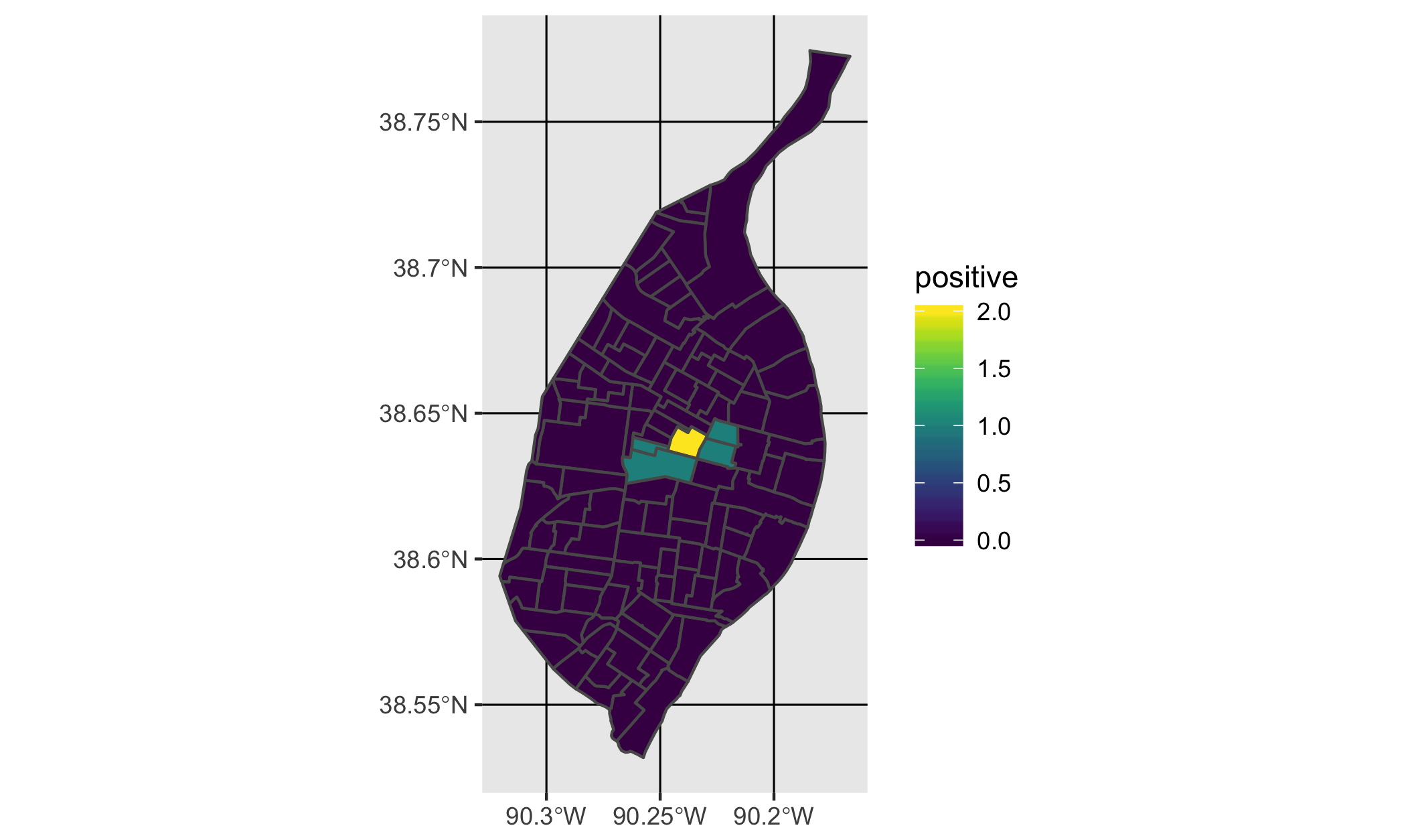
Mapping Summarized Data

Finally, we can use the geom_sf() geom from ggplot2 to map our summarized data, highlighting areas most discussed as being “positive” parts of St. Louis in our hypothetical study:

library(ggplot2)
library(viridis)

ggplot() + 
  geom_sf(data = qualData, mapping = aes(fill = positive)) + 
  scale_fill_viridis()

Since qualmap output are sf objects, they will work with any of the spatial packages that also support sf.

Getting Help

If you are new to R itself, welcome! Hadley Wickham’s R for Data Science is an excellent way to get started with data manipulation in the tidyverse.
If you are new to spatial analysis in R, we strongly encourage you check out the excellent new Geocomputation in R by Robin Lovelace, Jakub Nowosad, and Jannes Muenchow.
If you have questions about using qualmap, you are encouraged to use the RStudio Community forums. Please create a reprex before posting. Feel free to tag Chris (@chris.prener) in any posts about qualmap.
If you think you’ve found a bug, please create a reprex and then open an issue on GitHub.

Christopher Prener

2024-01-08